Setting up R
 A subdivision in the Crandon Drive and Peachwood Drive area in Charlotte, N.C. // Jeff Siner, The Charlotte Observer
The statistical programming language R is quickly becoming one of the standard tools for data journalists around the world.
In this walkthrough, you’ll learn how to:
- Install R and R Studio on your machine
- Install and import common packages
- Import data and generate simple summary stats
- Use keyboard shortcuts to save time
Installing software
There’s a variety of ways to work with R, which is the actual programming language. We’ll also use RStudio, a popular integrated development environment (IDE) that essentially functions as a user interface for the R language itself.
Step 1: Install R
Download and install the latest version of R from CRAN, the “Comprehensive R Archive Network,” for your operating system:
No need to change any of the settings in the default install wizard.
Step 2: Install RStudio
Download and install the latest version of RStudio (the website should automatically suggest the version for your operating system):
https://www.rstudio.com/products/rstudio/download/#download
Step 3: Open RStudio
To make sure everything is installed correctly, navigate to wherever your applications are stored and launch RStudio.
A few R basics
When you open RStudio for the first time, you’ll see a few different panes in your workspace. The largest is your console, which you can use to directly enter commands using the R language.
Execute the code by clicking Run or with Command + Enter.
Some commands, like simple arithmetic, are pretty obvious!
For the most part though, we won’t be working in the console directly. We’ll be writing our R code in an R script (a separate file we can save, reload and share) linked in an R project (which helps keep your data and scripts in one place in a working directory).
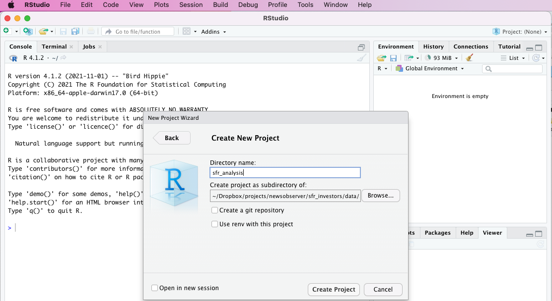
At the top menu, click File > New Project... and select “New directory, then New Project in the dialogue. You can specify where you want to store your project file and give it a name – we’ll use “sfr_analysis” – then click Create project.
After a few seconds, you’ll be mostly back where you started. One difference is the “Files” pane in the bottom right, which now shows your “working directory” – the folder where you chose to store your project. For now, this will probably only include your .Rproj file, which stores all the background data for your project.
Any files you add to this working directory on your computer will show up in this file viewer. It’s a nice way to keep track of your code and data and ensure things stay organized.
Now, on to creating a script.
At the top menu, click File > New File > R Script to start a new script. You’ll see your blank file appear in a new pane in RStudio. Go ahead and Save As... to give it a name. You should get in the habit of saving your work often.
At the top of your script, write a quick comment that tells you something about what your new script does. Starting each line with a # character will ensure this line is not executed when you run your code.
# R script for working with sfr data
# Created on 6/1/2022 by @mtdukes
You can do some simple arithmetic here again, like we did in the console. The only difference is that your code is saved, and you can run it again and again.
Code is executed line by line. Place your cursor on a line, then execute the line by clicking Run or with Command + Enter.
# doing some simple math
100 + 100
100 * 200
You can also store variables using an assignment function (<-). You can quickly insert these symbols with the keyboard shortcut OPTION + - .
The most basic variable types are characters, numerics, dates and logicals.
#store a numeric variable
current_year <- 2022

#store a date
current_date <- as.Date('2022-01-10')

#store a series of characters
current_month <- 'January'

#store a logical
is_winter <- TRUE
Installing and loading packages
R has a lot of great, basic functionality built in. But an entire community of R developers has created a long list of packages that give R a wealth of additional tricks.
We’ll harness some of those packages in our work analyzing the single-family rental industry.
One of the most popular packages is the tidyverse, a collection of utilties designed for data science. Let’s install a few of those packages.
Loading a package is a two-step process:
- Install the package.
- Load the package into your R workspace.
Installing is only necessary the first time you use a package. From then on, you’ll need to load the the package into your workspace only when you restart your project.
Execute each line of code by clicking “Run” or with CMD + Enter.
#install the tidyverse package
install.packages("tidyverse")
#install the tidyverse readxl package for loading Excel files
install.packages("readxl")
Then load them from our library, executing each line of code by clicking “Run” or with CMD + Enter.
#load our packages from our library into our workspace
library(tidyverse)
library(readxl)
Intro to the tidyverse
One benefit of tidyverse is the way it handles the import and processing of data in a specialized, easy-to-read dataframe, which is R’s parlance for a sequence of variables stored in a list. Think of a dataframe as a simple table with rows and columns.
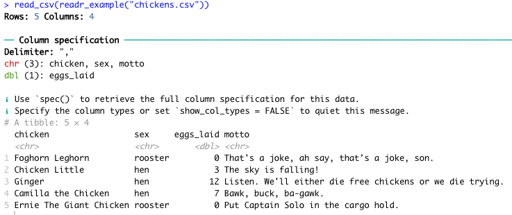
We can see that in action with a built-in example: a table of notable animated chickens (because why not).
#show a built-in dataframe of chickens
read_csv(readr_example("chickens.csv"))
Execute the code – by clicking “Run” or with CMD + Enter – to see the result print to your console.
Tidyverse also allows us to use the “pipe” – which looks like this: %>% – to chain together operations.
You can pipe the chicken data, for example, into the nrow() command to count the number of rows. When we execute code chained together with pipes, each chained-together runs in order from top to bottom.
#how many rows do we have?
read_csv(readr_example("chickens.csv")) %>% #load the data
  nrow() #count the rows
What’s the chicken count by sex? For that, we’ll use the count() function, which accepts one or more fields from our dataframe and… well… counts them.
If we want to know more about a function – for example, the syntax or what sorts of options is has – we can prepend a question mark to trigger the “Help” tab.
#what's up with the count function?
?count()
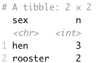
Let’s check the count by sex. This is something we can eyeball easily when the data is small, but it will come in handy when we’re dealing with hundreds of thousands of rows.
#count our chickens
read_csv(readr_example("chickens.csv")) %>% #load chicken data
  count(sex) #count by each variable in the 'sex' column
The summarize() function runs some math across a specified column in your dataframe. Think descriptive statistics: you can find out the sum, max or median across all values, for example.
#how many eggs laid on average?
read_csv(readr_example("chickens.csv")) %>% #load chicken data
  summarize(eggs_avg = mean(eggs_laid)) #calculate the average across the 'eggs_laid' column
It’s not surprising to note that our average here will be skewed by the roosters, which don’t lay eggs. So we can filter those out before we do our summary by chaining more commands together.
read_csv(readr_example("chickens.csv")) %>%  #load chicken data
  filter(sex == 'hen') %>% #only include hen rows
  summarize(eggs_avg = mean(eggs_laid)) #calculate the average across the 'eggs_laid' column
%>% symbol at the end of a highlighted section of code. Remember it chains your command to the next line, so RStudio will wait, thinking you're going to enter more code!Wrapping up
We’re just scratching the surface so far. But we should be all set to move forward with an analysis of your own property record data using tidyverse and a few other handy packages.