Looking for corporate ownership

A row of houses in a neighborhood impacted by corporate investors in Charlotte, N.C., on Feb. 7, 2022. // Khadejeh Nikoyeh, The Charlotte Observer

You’ve got your R project set up. You’ve cleaned your property owner names. And you’ve generated a custom lookup table.

Now it’s time to use what you’ve created so far to look for corporate ownership by matching the names in our property record database with the names in our lookup table using a join.

In this walkthrough, you’ll learn how to:

• Join two datasets in R
• Filter, group and count using the tidyverse
• Avoid common property record pitfalls
• Export data

NOTE: Don't forget about verification. Matches made with the techniques in this walkthrough – especially if you're using a lookup table customized for your state or cities – indicate a likely link to the corporate parents we're focusing on here. You'll need to confirm the relationship between subsidiary and parent in your own state, which may have very different companies than those we found in operation in North Carolina.

A primer on joins

A join is the process of uniting two datasets by matching them on one or more common variables. If this were a nice, tidy database, we might perform a join using a common ID number that indicates a definite relationship between the fields across our tables.

But we don’t have that here.

What we do have is a pretty good idea of how subsidiaries tied to corporate landlords are named across multiple regions. And we can use that knowledge to identify possible relationships between property owners in your data and the parent companies we identified in our investigation.

Instead of matching an ID number, we’ll attempt to match the data using the clean name from your property record database and the owner_name from our investors_clean data (our lookup table).

There are lots of types of joins, but for this analysis, we’ll use a LEFT JOIN. Which looks like this.

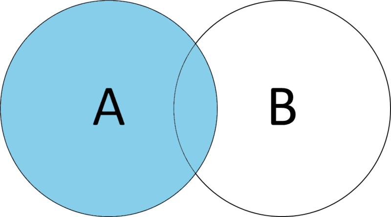
Our property record data is our left table (Table A in the example below), and our parent company lookup table is our right table (Table B in the example below).

Executing a left join using owner names means that only columns from our parent company lookup table that match will be tacked on to our property owner data.

Joining our data

Tidyverse’s left_join() function accepts a dataframe (your property records table, in this case) and a by parameter, which tells the function what we actually want to match on.

In this case, the column names we want to match are different.

That’s OK! We just use the left table’s column name on the left of the equal sign, and the right table’s column name on the right of the equal sign.

In our case, we’re using our clean-up property data from Wake County (stored in wake_properties_clean). You’ll need to modify the code below to join your specific market’s data (both the table name and the property owner name variable)

#join our cleaned property data with our lookup table
wake_properties_labeled <- wake_properties_clean %>% 
  left_join(
    investors_clean, by = c('OWNER1_clean' = 'owner')
  ) %>% 
  relocate(investor_label_lvl1, investor_label_lvl2, .after=OWNER1_clean)

After a few seconds, you should see your new table added to your list of data entries in your Environment pane in the top right of R Studio.

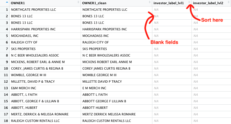
If you double-click to open that dataset, it might not appear very successful on first glance. In our version, for example, the first 20 or so rows show blank entries for investor_label_lvl1 and investor_label_lvl2.

That goes back to the type of join we used.

A left join keeps our left table (our property records) intact, so rows that don’t match our lookup table come over as blank, or NA.

You can do a quick gut check to see if anything matched by clicking the arrows in the investor_label_lvl1 column in the table view pane to sort the data.

If you got a match (or many), you should see cells with “INVESTOR” filled in the investor_label_lvl1 column. Next, we’ll find out exactly how many.

NOTE: Not seeing any matches? Check your code. Are you joining the correct tables? Did you identify the correct field names? Are you matching on the cleaned versions of the fields?

Quantifying corporate ownership

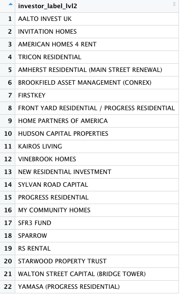
You may have noticed that there are two “levels” to our investor labels. One just says “INVESTOR”, while the other gets more specific about one of more than 20 companies we focused on for our reporting.

You can get a quick look at those companies by examining the lookup table itself.

# examine which companies are contained in our lookup table
investors_labeled %>% 
  distinct(investor_label_lvl2) %>% 
  view()

Let’s see if we can get a sense of just how many properties these companies own.

We can do that with the filter() function, showing only rows with the “INVESTOR” label, then counting them with nrow().

#how many properties did our join identify
wake_properties_labeled %>% 
  filter(investor_label_lvl1 == 'INVESTOR') %>% 
  nrow()

If we want to examine those rows in their own more manageable table, we can largely repeat the code, assigning the output to a new dataframe.

#store investor-ided properties in a new dataframe
wake_sfr <- wake_properties_labeled %>%
  filter(investor_label_lvl1 == 'INVESTOR')

We can also get a breakdown of these properties by company with the count() function, which we arrange in descending order.

#break down properties by company
wake_sfr %>% 
  count(investor_label_lvl2) %>% 
  arrange(desc(n))

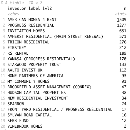
In Wake County, N.C., this technique has identified more than 5,400 properties likely owned just by these companies as of data accessed in early June 2022.

Pitfalls to avoid

We’ve noted the importance of verification several times in these walkthroughs. And although there’s a good deal of fact-checking required to confirm the connections between our subsidiaries and their parent companies, it also important to understand potential issues with property record data.

Your particular property record data will be specific to your state or city, so it pays to find local experts who can tell you about issues to avoid – or even who would be willing to eyeball your preliminary findings.

But there are a couple of issues we ran into that appear to be fairly common.

Duplicate parcels

Property/parcel databases can be messy for a variety of reasons, chief among them that they’re maintained by fallible human beings who are keeping track of a lot of information dating back a very, very long time.

As a result you may find that some rows are duplicates. That’s bad, because it could potentially inflate your count. But there are rows that might initially seem like duplicates that actually describe something different – for example, multiple structures on the same plot of land.

A few important questions you should answer:

• Does your property data describe parcels or buildings?
• Does your data have a real estate identification number, or a parcel identification number?
• Does that real estate ID or parcel ID describe the parcel or the building?
• Should that real estate ID or parcel ID be unique?

When you find a unique ID number, you can analyze how often that number is repeated in your data to root out potential duplicates.

#count the number of distinct rows
wake_sfr %>% 
  distinct(Parcel_Identification) %>% 
  nrow()

#identify any duplicate parcel ids in a table by count
wake_sfr %>% 
  count(Parcel_Identification) %>% 
  filter(n > 1) %>% 
  arrange(desc(n))

In our case, there are no duplicate parcel IDs in Wake County. But that’s an issue you want to make sure you address before you publish.

Buildings that aren’t single-family homes

Some, but not all, of the major players in the single-family home rental industry also dabble in other types of rentals – townhomes, condominiums, even multi-unit apartment buildings.

It’s possible you’re interested in ownership of all these different types of rentals. But that decision matters if you’re trying to get a sense of the percentage of homes these companies own in a neighborhood, city, county or state. It changes your denominator, so make sure you come up with a clear and documented definition so you can explain how you drew your conclusions.

In our case, we were interested in single-family homes that fit the definition from the U.S. Census Bureau:

The single-family statistics include fully detached, semidetached (semiattached, side-by-side), row houses, and townhouses. In the case of attached units, each must be separated from the adjacent unit by a ground-to-roof wall in order to be classified as a single-family structure. Also, these units must not share heating/air-conditioning systems or utilities. Units built one on top of another and those built side-by-side that do not have a ground-to-roof wall and/or have common facilities (i.e., attic, basement, heating plant, plumbing, etc.) are not included in the single-family statistics.

To make sure we weren’t sweeping up any non-single-family properties in our data, we consulted the data dictionary and used both zoning and use codes to weed out properties that didn’t fit, given us the most conservative possible estimate we knew we could stand behind.

In Wake County, that field is called TYPE_AND_USE, and we can use our count() function again to examine the breakdown.

#break down by type and use code
wake_sfr %>% 
  count(TYPE_AND_USE) %>% 
  arrange(desc(n))

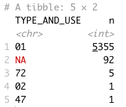
The vast majority, as we can see, are properties with the “01” code, which corresponds to “RESIDENTIAL - ONE FAMILY”, per the county’s code description document.

That’s a relief!

We can safely exclude the handful that don’t fit our definition.

As for the NAs, or blanks, we could filter them out or spot check them – we found in many cases, this indicated new construction or were pretty reliably single-family homes where the code just wasn’t entered.

Check for these inconsistencies to avoid drawing incorrect conclusions that will force corrections down the road.

Once you’ve identified the issues, you can take a final cleaning step to remove what you don’t want and store the result in another dataframe.

#deduplicate and filter only single-family properties in the data
wake_sfr_final <- wake_sfr %>%
  distinct(Parcel_Identification, .keep_all = TRUE) %>% 
  filter(TYPE_AND_USE == '01')

Wrapping up

If you want to share the data – or use it in other platforms or software – you can easily export it into a CSV file. It’s also a good habit to timestamp your file so you can differentiate it from other versions – say if you find other problems or pull new data.

#export the data into csv with a auto timestamp
wake_sfr_final %>% 
  write_csv(paste0('wake_sfr_properties',
                   format(Sys.time(),'%Y%m%d%H%M'),
                   '.csv'))

You should see now see your data in your working directory.

There’s plenty of reporting left to do here, obviously.

And it’s important to note that our list of companies doesn’t represent the totality of the corporate single-family rental industry. In fact, some of these companies aren’t represented by the National Rental Home Council, the trade group that represents some of the largest players in the business.

Our analysis, as our methodology notes, excluded companies with fewer than 100 properties in their North Carolina portfolios, as of data collected and analyzed in April 2022.

But this should give you a good start.